Repeated Measures

First, we will want to read our data into R. The data, called ThreeTimePoint.sav, are in the SPSS (.sav) format. In order to read data in the .sav format into R, we need to use a function that is available in the

foreign

library. Load the library and read in the data using the following commands.

> library(foreign)
> depression=read.spss("ThreeTimePoint.sav", to.data.frame=T)
> attach(depression)

Next, we will examine the data.

> depression
BEFORE AFTER FOLLOWUP
1 2 3 5
2 4 7 9
3 6 8 8
4 8 9 8
5 10 13 15
6 3 4 9
7 6 9 8
8 9 11 10

Data Exploration: State Education Data

Again, we will want to read our data into R. The data, called StateEducation.sav, are in the SPSS (.sav) format. In order to read data in the .sav format into R, we need to use a function that is available in the

foreign

library. Load the library and read in the data using the following commands.

> library(foreign)
> education=read.spss("StateEducation.sav", to.data.frame=T)
> attach(education)

Next, we will summarize the B2005 variable by finding the mean and median.

> mean(B2005)
[1] 27.35098
> median(B2005)
[1] 25.8

To obtain the trimmed mean, we add the argument

trim=x

to the

mean

command, where x is the fraction (0 to 0.5) of observations to be trimmed from each end of the data before the mean is computed.

> mean(B2005, trim=.2)
[1] 26.84194

Unfortunately, R does not have a native function to compute the winsorized mean. To obtain the winsorized mean, we have to create our own function. You can copy and paste the following lines of code into R.

win<-function(x,tr=.2){
#
# Compute the gamma Winsorized mean for the data in the vector x.
# tr is the amount of Winsorization
#
   y<-sort(x)
   n<-length(x)
   ibot<-floor(tr*n)+1
   itop<-length(x)-ibot+1
   xbot<-y[ibot]
   xtop<-y[itop]
   y<-ifelse(y<=xbot,xbot,y)
   y<-ifelse(y>=xtop,xtop,y)
   win<-mean(y)
   win
}

To obtain the Winsorized mean we can now employ the function that we just put into R.

> win(B2005, tr=.20)
[1] 26.94314

Both the variance and standard deviation can be obtained in R by using the following syntax.

> var(B2005)
[1] 33.22055
> sd(B2005)
[1] 5.763727

To obtain a robust estimate of the variance of the trimmed mean - which can be based on the Winsorized sum of squared deviations - we will again copy and paste the following function into R.

winvar<-function(x,tr=.2,na.rm=F){
#
# Compute the gamma Winsorized variance for the data in the vector x.
# tr is the amount of Winsorization which defaults to .2.
#
   if(na.rm)x<-x[!is.na(x)]
   y<-sort(x)
   n<-length(x)
   ibot<-floor(tr*n)+1
   itop<-length(x)-ibot+1
   xbot<-y[ibot]
   xtop<-y[itop]
   y<-ifelse(y<=xbot,xbot,y)
   y<-ifelse(y>=xtop,xtop,y)
   winvar<-var(y)
   winvar
}

We can then find the Winsorized variance and for the B2005 data by using,

> winvar(B2005)
[1] 8.514902

To get the standard error for the mean we can employ the formula from the notes as,

> sd(B2005)/sqrt(length(B2005))
[1] 0.8070832

The robust estimate of the standard error for the trimmed mean can be obtained by again copying and pasting the following formula into R

trimse<-function(x,tr=.2,na.rm=F){
#
# Estimate the standard error of the gamma trimmed mean
# The default amount of trimming is tr=.2.
#
   if(na.rm)x<-x[!is.na(x)]
   trimse<-sqrt(winvar(x,tr))/((1-2*tr)*sqrt(length(x)))
   trimse
}

Then entering the following command.

> trimse(B2005, tr=.2)
[1] 0.68101

To obtain the mean plot and the mean plot with error bars, we need to use data that is in a different format. This data has been reformatted and is available as StateEducationlongFormat.sav. Read in this data and load the

gplots

library using the following commands.

> education2=read.spss("StateEducationLongFormat.sav", to.data.frame=T)
> library(gplots)

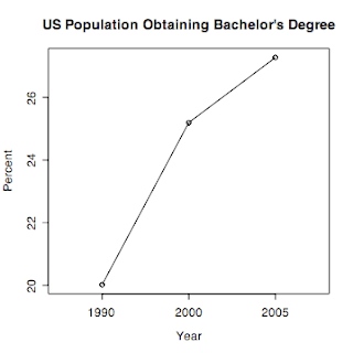
The mean plot can be obtained by entering,

> plotmeans(BACH~YEAR, data=education2, connect=T, p=0, n.label=F, xlab="Year", ylab="Percent", main="US Population Obtaining Bachelor's Degree")

The mean plot with error bars can be obtained by modifying the

p=0

argument to

p=.95

as follows,

> plotmeans(BACH~YEAR, data=education2, connect=T, p=.95, n.label=F, xlab="Year", ylab="Percent", main="US Population Obtaining Bachelor's Degree")

Data Exploration: Vietnamese Age Data

The first thing we will want to do is read our data into R. The data, called VietnameseAgeData.xls, is in the Excel format. In order to read data in the .xls format into R, we need to use a function that is available in the

gdata

library. Load the library and read in the data using the following commands.

> library(gdata)
> ages<-read.xls("VietnameseAgeData.xls")
> attach(ages)

The

attach

command attaches the dataset to the searchpath so that we only have to give the variable name rather than call the dataset each time. Next, we will examine the data.

> names(ages)
[1] "age"
> age[1:10]
[1] 68 70 31 28 22 7 57 27 23 0
> length(age)
[1] 28633
> summary(age)
Min. 1st Qu. Median Mean 3rd Qu. Max.
0.00 12.00 23.00 28.14 41.00 99.00

Graphically, we want to examine a histogram of the data. The four histograms in the notes are replicated using the following commands

> par(mfrow=c(2,2))
> hist(age, breaks=55)
> hist(age, breaks=40)
> hist(age, breaks=25)
> hist(age, breaks=10)
> par(mfrow=c(1,1))

To obtain the plots of the kernel density estimates, the following R commands were used.

> par(mfrow=c(2,2))
> plot(density(age, kernel="epanechnikov", bw=.5), main="")
> plot(density(age, kernel="epanechnikov", bw=2.344), main="")
> plot(density(age, kernel="epanechnikov", bw=5), main="")
> plot(density(age, kernel="epanechnikov", bw=10), main="")
> par(mfrow=c(1,1))

Introduction

This blog is intended to introduce students enrolled in EPsy 8261 and EPsy8262 to the statistical software R by working through the examples provided in the lecture notes. All of the data sets are available on the course websites for EPsy 8261 and EPsy 8262.

To obtain R and get started visit the Comprehensive R Archive Network. The blog entries will primarily offer the code needed to replicate the results and figures in the class notes. As time permits, more exposition and direction may be added. There are many wonderful tutorials available on R floating about the web if you want additional information.